Scope
Scope
Overview
The scope allows you to plot up to six different parameters from the drive. Use Full View and Normal View to toggle between the scope setup (normal) and a larger view of only the scope output (full). You can configure, save, and restore scope settings from the normal view. The lower right corner of the normal view also includes a box that indicates status, drive and scope control buttons (Stop Motion, Enable Drive, Start Recording, and Refresh).
Using the Scope
You can set up scope plots using the tabs summarized below:
|
Tab |
Function |
|---|---|
|
Select data source, plot axes, and plot appearance. |
|
|
Select how much data to record and when to start recording the data. |
|
|
Defines traces to calculate based on two existing channels. |
|
|
Generate basic motion. |
|
|
Use motion tasks for motion. |
|
|
Set the loop gains for axes |
|
|
View all current tuning gains in the drive and manually edit gains. |
|
|
Adjust filter settings. |
|
|
Save or print the plot as an image. View, save, or print the raw data. |
|
|
Display basic statistics of the data. |
|
|
Turn on the cursors and view the data at the cursor positions. |
|
|
Pan, zoom, and control the grid and background color. |
|
|
Configure presets and y-axis group settings. Save, import, or export settings. |
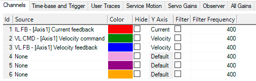
Channels
The Channels tab allows you to select and record up to six channels simultaneously. Select the data to record for each channel (see Keyword Picker for more information on how this can be done very easily). You can also set the Color for each channel, the Y-axis data type, and Filter and Filter Frequency columns. Once a recording is shown on the Scope view, you can click Hide to remove a channel from the Scope display.
|
Feature |
Description |
|---|---|
|
Source |
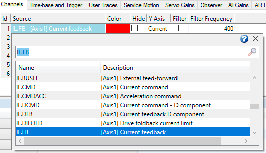
To set a channel to record, click the source you want to set and choose the appropriate channel. You can choose from None (no data is collected on that channel), preset trace types, or enter a user-defined trace. Choosing “<User Defined>” allows you to record data from pre-defined locations. These locations are provided by the factory to collect less common values. See the screenshot below for additional context. |
|
Color |
Select a color to change that plot trace's appearance in the Scope view. |
|
Hide |
Check the Hide box to remove a given plot trace from the display. This feature can make it easier to focus on specific traces. |
|
Y-Axis |
Choose which Y-axis the channel displays. Several predefined Y-axis groups exist. Click on the item in the column to change the label for the trace. |
|
Filter / Filter Frequency |
Check the Filter box and use the frequency column to apply a low pass filter to the data collected. The filter is applied when data is collected, and will not be applied to data collected prior to checking the box. |
Source
Time-base and Trigger
-
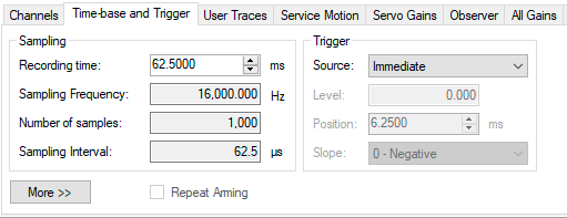
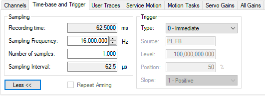
Use the Time-base and Trigger tab to select how much data to record and when to start (trigger) recording the data. You can set length of recording in ms and the sampling frequency in Hz. The number of samples is a calculated value displayed for reference.
-
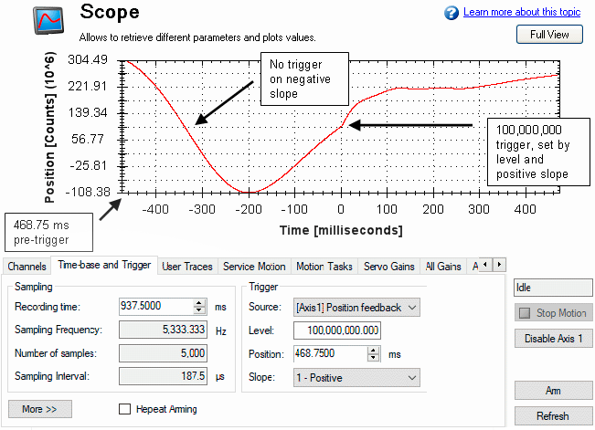
The trigger can be set to trigger immediately when you click Start Recording or to trigger when a specified value for a given signal is reached. The default Time-base and Trigger view specifies recording time, sampling frequency, and either an immediate trigger or a trigger based on one of many predefined sources.
-
Click the More button in this view to specify a given number of samples, sampling frequency, sampling interval, and access additional trigger options.
If you choose a source other than Immediate, you can set the level, position, and slope for the trigger value.
- Level sets the value of the source that triggers the recording to start.
- Position sets the amount of time the scope displays before the trigger occurred.
- Slope sets whether the source data must pass the level value in a positive or negative direction.
More
Toggle the More button to display additional options for configuring the time-base and trigger.
Less
The default options for configuring the time-base and trigger are shown when the Less button is displayed.
Sampling
In the Sampling area of this view, you can specify the recording length by entering a sampling frequency and a number of samples. Here, the recording time is a calculated value displayed for reference.
What is triggering?
Triggering allows you to precisely control the start point of data collected in the scope. For example, if you are looking for a large spike, you can set the trigger to start the scope to begin recording when it sees the large spike. This section describes the triggering functionality of the scope.
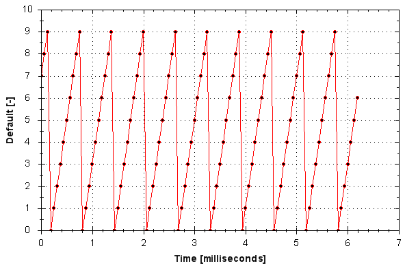
Test Signal
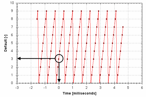
As an example, it is useful to examine variations on a record of a test signal that generates a sawtooth signal. The signal starts at 0 and increases by one every drive sample (1/16,000 second) to a maximum of 9, and then returns to 0. This signal continues indefinitely. The record of this signal is shown below.
Trigger Type
The Trigger area in the More view offers more flexibility than the default view. You can specify six types of trigger types
|
Type |
REC.TRIGTYPE Value |
Description |
|---|---|---|
|
Immediate |
0 |
This mode will start recording as soon as the recording command |
|
Next Command |
1 |
This trigger type lets you specify a trigger on the next telnet command received by the drive. This is useful in a telnet session via Hyperterminal or a similar program. WorkBench is constantly sending telnet commands, so this is not typically used in a WorkBench session. |
|
Signal On Edge |
2 |
This trigger type lets you specify a trigger source and set of conditions to trigger recording of data. This is similar to the triggering used on oscilloscopes. |
|
Signal On Boolean |
3 |
This trigger type lets you trigger on a boolean (0 or 1), such as drive active status. The scope triggers when the source equals what the slope indicates: 1 if the slope is positive and 0 if the slope is negative. |
|
Signal on Value |
4 |
This trigger type specifies that the signal has to exactly match the specified trigger value. |
|
Signal on Boolean w/ Mask |
5 |
This trigger type specifies that the signal ANDed with the trigger mask |
The Bitmask type has a mask input to the right of the trigger type. Otherwise, you can specify the mask using the keyword
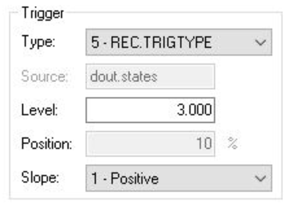
If we want to trigger when both DOUT1 and DOUT2 are set, we can set
Trigger Position
Trigger Position
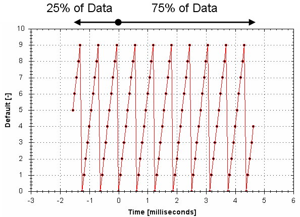
Trigger position is specified in units of percent (%). If you specify a trigger position of X% , X% of the data is before 0 ms in the data time and 100-X% (the rest of the data) is at or greater than 0 ms. In the picture below, trigger position is set to 25%
In the WorkBench scope, the 0 time point is clear. When collecting the data via REC.RETRIEVE or similar commands, the time is not returned, so some caution should be used when the trigger point is important to understand.
Trigger position is not used in trigger type “Immediate” (TRIGTYPE 0).
Trigger Value
The trigger value
The trigger value is not used in the Boolean trigger type. Use the trigger slope to set the polarity of the Boolean trigger.
The trigger value is just a number and has the units of the source signal.
- The trigger source is less than the trigger value in the previous recording sample
- The trigger source is greater than or equal to the trigger value in the current recording sample
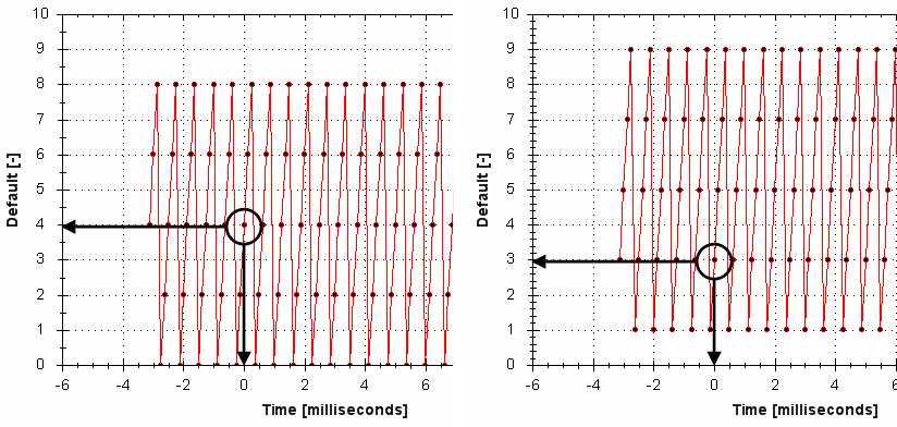
Below is an example showing triggering of trigger value of 3
When the trigger slope is negative
- The trigger source is greater than the trigger value in the previous recording sample.
- The trigger source is less than or equal to the trigger value in the current recording sample.
Effects of Recorder Gap
When the recording rate is less than 16,000 Hz
- You cannot be sure of the moment that the recorder is triggered any closer than N samples. An example of this is shown below where the trigger value is set to 3, the trigger slope is positive and the recorder gap is 2. Both examples used the same data, but the first graph
- You can miss triggers, whose duration is less than N samples, where N is the value of
A workaround for the above effects is available by setting the recorder trigger position to zero
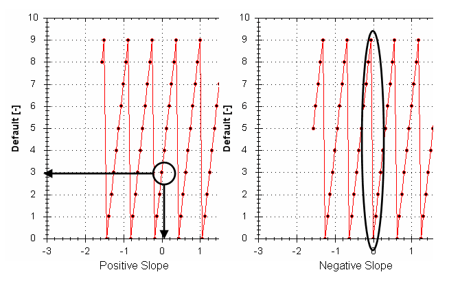
Trigger Slope
Trigger Slope specifies whether you trigger on a positive or negative change in the trigger source. The effect of the trigger slope is different for trigger type Boolean and On Next Signal modes.
Boolean Trigger Type
When using Boolean type:
- A positive slope will trigger when the trigger source is 1
- A negative slope will trigger when the trigger source is 0
The boolean trigger type is a state trigger. There is no need to transition from 0 to 1 to trigger with the positive slope. If the trigger source is 1 from the start, the positive slope will immediately trigger.
On Next Signal Trigger Type
The “On Next Signal” trigger type allows you to specify if the recorder should trigger when the signal crosses the trigger level in the positive or negative direction. The signal only needs to reach the trigger level; it does not need to pass the trigger level.
In the examples below, the trigger value is set to 3
User Traces
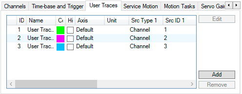
The User Traces tab is used to create a custom trace calculated from the data of two sources, with each source containing either a channel or previously declared user trace.
-
- A user trace can only reference another trace declared before itself.
Add and Configure a User Trace
From the User Traces tab, select Add.
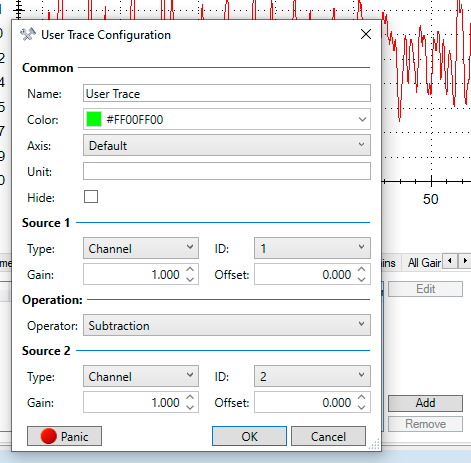
The User Trace Configuration will multiply, divide, add, or subtract the data of the two selected sources.
| Setting | Description |
|---|---|
| Name | Name to display in the scope for this trace. |
| Color | Color of the trace in the scope. |
| Axis | Defines the y-axis the trace is drawn on. Choose from an existing axis or from a custom axis created from the Settings tab. |
| Unit | Custom string defined by user. This string is only for user tracking and has no effect on any units. |
| Hide | Check to hide this trace from the scope. |
| Source 1 and 2 | These constitute the two operands of the calculation to be performed. |
| Type:ID, Gain, Offset | Select either an existing channel or previously declared user trace to be used in the calculation. The gain and offset are also configurable and will be calculated as Gain*(Type:ID + Offset). |
| Operator | Choose the type of calculation (Addition, Subtraction, Multiplication, Division) to be performed. |
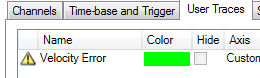
Select Ok after configuring, and the custom trace will be added to the scope. Defining a custom y-axis (in the Settings tab) allows the trace to be shown on a different scale. In the example below, Velocity Error is a User trace of VL.CMD - VL.FB shown on the axis named Custom, while VL.CMD and VL.FB are shown on the Velocity axis.

If a User Trace points to invalid data, it will not draw the data in the scope and a warning sign will appear. Check your Ch. IDs of your User Trace and the channel sources in the Channels tab to make sure both are properly configured.
Saving User Traces
User traces can be saved for later use when creating a new preset.
-
- User traces will not be saved when saving a csv file from the Save and Print tab. Only the channels from the Channels tab will be saved to the file.
Service Motion
The Service Motion tab provides almost the same interface as the Axis-level Service Motion screen. The main difference is that both axes are represented by vertically aligned tabs on the left side of the screen. For all other details, please refer to the Service Motion Screen. This tab provides a compact view of all the elements of Service Motion.
Motion Tasks
This tab contains all the active motion tasks for Axis 1 and 2.
Servo Gains
This tab provides a convenient way of setting the loop gains for both axes.
All Gains
This tab contains all the gain settings in the drive.
AR Filter
This tab contains the Anti-resonance filter settings.
Save And Print
This tab is useful to record the displayed data (or to display pre-recorded data). If you want to save the viewable image you can use the button "Save Image As..." which allows you to choose the various image formats. Similarly you can use the button "Save csv File..." to save all the recorded data in CSV format. You can also Email the image or the CSV file or launch Excel to read the CSV data. The User Note space allows you to store notes and associate it with the saved data. WIth the button "Load csv File...", you can also load data from a recording that was previously captured.
Measure
This tab shows you statistics about the data that was recorded for each of the channels: Average, Minimum, Maximum, Peak to Peak, True RMS, AC RMS and the Units.
AC RMS and True RMS
In the measure tab, there is a column for AC RMS and a column for True RMS. True or full RMS is the more correct RMS value of a signal and includes any DC terms in the value. AC RMS removes DC components and gives only the RMS value as a measure of a signal's standard deviation.
True RMS = Sqrt{Sum(x[n]^2)/N} where N is number of pointsAC RMS = Sqrt{(True RMS)^2 - (dc or average value)^2}
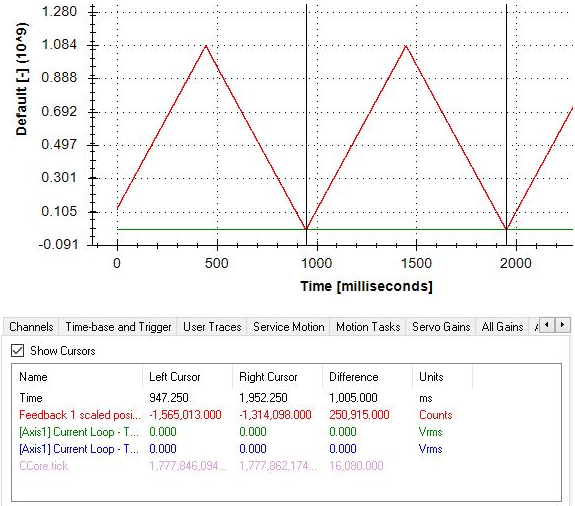
Cursors
This tab allows you to measure inflections in the recorded signal and measure the values at the two cursor positions. To make the cursors visible, check the "Show Cursors" box as shown below. Then, drag and drop the cursors as shown below to measure the distance between the sawtooth troughs.
Display
The Display tab allows you to move and size the visible area of the scope graph. It also allows you show or hide the grid, and other miscellaneous features. The checkbox "Show Data" allows you to show the data without launching Excel if you want to quickly view the data.
Settings
Scope settings are used to store and retrieve the scope parameters. You can save multiple settings, called "presets", under different names. You can save, delete, import, or export the presets. The settings are stored in WorkBench project file (default.wbproj) and settings are common to all the drives in WorkBench.
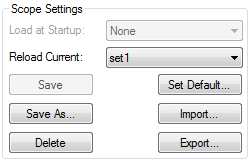
Load a Setting (Preset) to Scope
In Scope Settings section, the existing presets are listed in the Select Setting box. To load a setting to the scope screen, select the desired preset from the Select Setting list.
Create a New Preset
- Modify any scope parameters.
- Select the Settings tab.
- Click Save As. The following dialog is displayed:
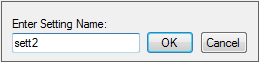
- Enter the setting name and click OK. The current settings are saved as a preset with the given name and displayed in the list.
Save or Delete Preset
Save saves any modification to the open preset. Delete deletes the open preset.
Import a Preset
Import the presets contained in the selected settings file as follows:
- Click on Import button and the following dialog will be displayed.
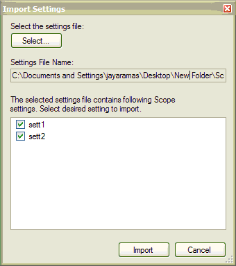
- Select the settings file by clicking “Select…” button.
- All the scope presets will be displayed contained in the selected settings file.
- Select/Deselect the presets and then click on Import.
- If preset name already exists in application the confirmation message will be shown to user to replace it or to ignore.
Export a Preset
Export a preset to a file as follows:
- Click Export and the following dialog is displayed:

- The existing presets are displayed and user can select/deselect the preset to export.
- Select the file name to export.
- Click Export to export the selected presets to a file.
Scope Axis Scaling and Zooming
The scope provides two mechanisms for determining how you view the data:
- Scaling: you can choose the scale for the different axes.
- Zooming: you can choose a particular portion of the scope that you want to observe more in details, and then come back to previous scaling.
Two different scaling modes are provided on each axis:
- Manual: you can determine the minimum and maximum value of the axis (X or Y axis).
- Scale to fit: the program will compute a scale for this axis that will display all the curves bound to it (X or Y axis).
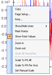
These functionalities are accessible through the contextual menu when right-clicking in the axis zone. A simple left-click in the axis zone will provide the manual range functionality. A supplementary functionality allows you to perform a scale to fit on all axes is also available, which allows a good overview.
The zoom functionality allows you to navigate in a portion of the graphic. When you reset the zoom, the initial scales are shown.
In the display tab, when “Remember Axis Scale” is set, the scales of the axes are kept between two sequential recordings. You can fine tune the scale to visualize a particular behavior and record a second time and see the same behaviour without having to redo all the tuning. When not checked, a scale to fit all will be performed after each record. This setting is reseted when exiting WorkBench and should be explicitly set at next startup.
Manual Range Per Axis
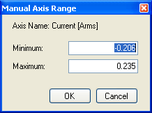
After recording data, right click anywhere on the y-axis and select Set Manual Scale to open a dialog box to set the range for the axis. Enter the Y-axis minimum value and Y-axis maximum value. Click OK to reset the Y-axis to new range.
Unit Display on Y Axis
The unit on the Y-axis is displayed if all scope signals units are identical for that Y-axis. If different units apply to different signals, the units are displayed as [-]. For example, if the velocity Y-axis has signals VL.FB and IL.CMD, then the unit displayed is [-], since the units for these parameters are different. If IL.CMD is hidden, then the correct unit for VL.FB, rpm, is displayed.
Related Parameters: