


The Performance Servo Tuner (PST) can be set up to use specific modes or limits in tuning to provide tuning in ways you can control, while still taking advantage of the PST’s ability to make decisions quickly and effectively for you.
To use the advanced modes of the PST, click the More button to display the additional features for advanced autotuning:
Typical Cases for Advanced PST Use
Tuning Systems with Low-Frequency Resonances
Systems with low-frequency resonances are challenging because low frequency data is difficult to measure. While the PST can tune these systems, you can expect lower system performance. If your system has a first anti-resonance of 30 Hz (pictured below), you can expect approximately 15 Hz (half the frequency of the first anti-resonance) of closed loop bandwidth.
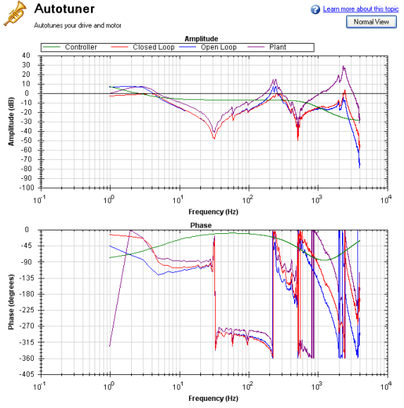
In addition, in order to accurately measure the low frequency resonances, the fast Fourier transform (FFT) resolution must be sufficiently fine to accurately measure the low-frequency resonance. A good place to start is to have an FFT resolution of 1/10 of the frequency of the lowest anti-node. In the case shown above, an anti-resonance of 30 Hz is present, so the resolution should be approximately 3 Hz FFT resolution. The PST can function with the resonance if it is accurately measured, as shown below. To adjust the FFT resolution, adjust FFT Points in the Recording Options tab as needed.
Tuning Systems with High-Frequency Resonances
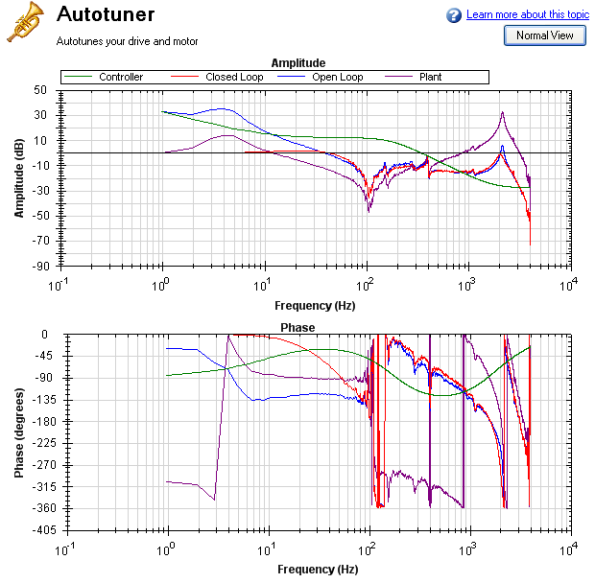
Some systems have resonances at very high frequencies (greater than 1 kHz). When the resonance is this large, it can prove a challenge in tuning, because these systems generate high noise levels that are often audible. An example of a large resonance is shown below. This example is from a steel flywheel mounted to an AKM22E
One way to resolve this problem is to use a low-pass filter in the feedback path. To use this filter, check the Enable Lowpass Search in the PST, which is the default behavior.
Tuning systems with noisy frequency responses
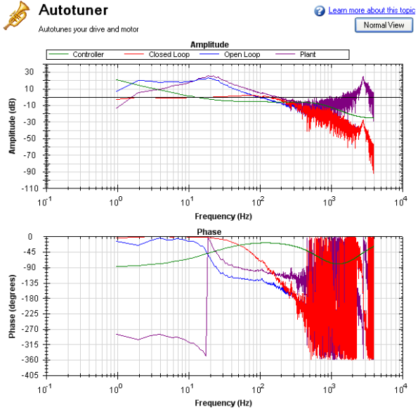
When using a motor with a low-resolution incremental encoder or resolver, the high frequency response may be noisy. Below is a Bode plot created after autotuning of an incremental encoder with 8,192 counts per revolution.
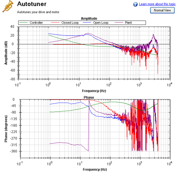
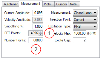
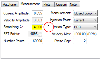
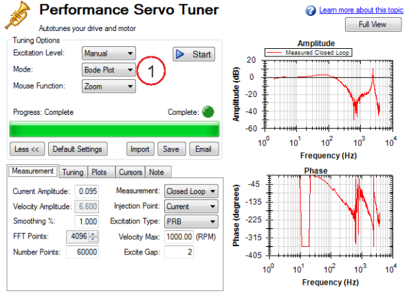
To make the Bode plot easier to read, increase the smoothing factor (1) in the advanced Measurement
Options.
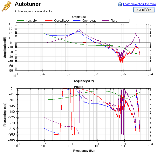
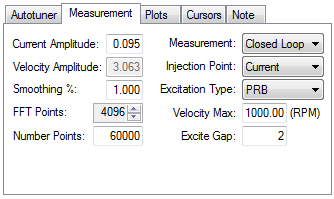
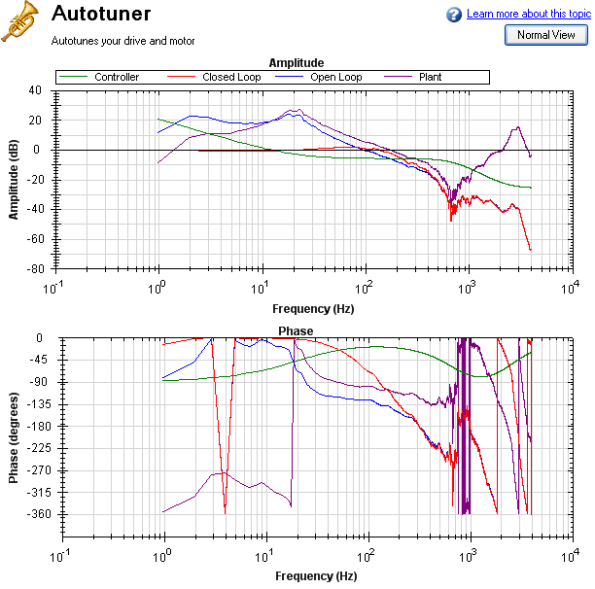
After increasing the smoothing percentage, the Bode plot traces become cleaner and easier to read:
PST Options
When you click More in the PST view, the following options are displayed:
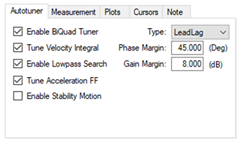
Enable BiQuad 1 Tuner
Check this box to use the first anti-resonance filter in the forward path (AR1). You can specify the type of filter to use in the Type box to the right of Enable BiQuad 1 Tuner.
Enable BiQuad 2 Tuner
Check this box to use the second anti-resonance filter in the forward path (AR2). You can specify the type of filter to use in the Type box to the right of Enable BiQuad 2 Tuner. Enabling this option may significantly slow your computer during this operation.
Biquad Type
For Biquad 1 and 2, you can choose what type of filter to implement. The four options are:
- LeadLag: The LeadLag filter is the default, and will work for most servo systems.
- Lowpass: A Lowpass filter requires the least amount of processing time. The PST will place the lowpass to get the maximum bandwidth possible.
- Resonator: The Resonator filter is like a Notch filter with tunable bandwidth and notch depth. The Resonator takes longer to calculate than the LeadLag filter.
- Custom: The Custom filter takes the longest to calculate and does not restrict the PST to a filter shape. This filter type provides excellent results, but may significantly slow your computer while the filter is calculated.
Tune Acceleration FF
This box turns on and off the acceleration feedforward tuner. If this box is checked, the PST will measure the inertia attached to the motor shaft, and using this measurement, will calculate an appropriate acceleration feedforward and write it to the drive
Enable Stability Motion
When this checkbox is checked, after the PST has completed, the PST will command a short move in the clockwise direction, then back to its origin and monitor the motor's parameters to determine if the tuning is stable. If an instability is detected, the drive will generate Fault F6003 : Instability during Autotune.
The PST always ensures that the tuning satisfies stability criteria that can be adjusted in units of phase margin (in degrees) and gain margin (in dB). The PST uses default values for phase and gain margin, but you can adjust these values to ensure higher stability or to allow the PST to be more aggressive by using lower gain and phase margins.
Tune Velocity Integral
Check this box to tune
Enable Low Pass Search
Check this to tune a fourth-order low pass filter in the feedback path (AR 3 and 4). If this box is unchecked, the PST will not modify the anti-resonance filters in the feedback path.
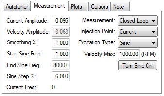
Measurement Options
The PST screen also provides options for measurements:
Current Amplitude
This box sets the amplitude of the current used to excite the system during a current injection mode excitation. This amplitude applies to all excitation types when the Injection Point is set to Current. The Current Amplitude box is disabled if the Injection Point is set to anything else.
Velocity Amplitude
This box sets the amplitude of the velocity used to excite the system during a velocity injection mode excitation. This amplitude applies to all excitation types when the Injection Point is set to Velocity. The Velocity Amplitude box is disabled if the Injection Point is set to anything else.
This value applies a moving average smoothing filter to the frequency response gathered during autotuning. This process reduces noise in the frequency response that can occur when making short frequency response measurements, using low resolution encoders, conducting low amplitude frequency response tests, or for other reasons. The smoothing filter iterates through each frequency on the FFT plot. For each frequency, all frequencies within the Smoothing % range will have their magnitudes averaged.
For example, if you smooth a Bode plot with 5% smoothing, at 100 Hz, it will average all the values between 95Hz and 105Hz; when the filter gets to 1000 Hz, the filter will average all the values between 950 Hz and 1050 Hz.
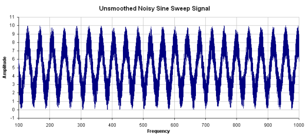
As an example, assume a noisy sine sweep signal and use a 5% smoothing factor. Below is a noisy signal with a range of 100 Hz to 1000 Hz.
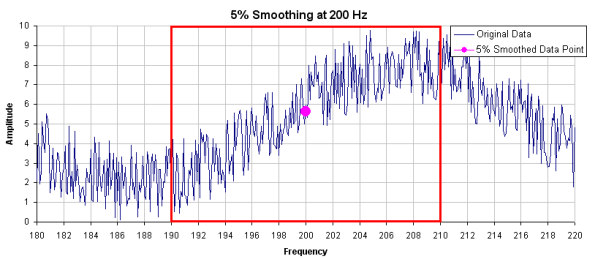
In this example, examining how the smoothing filter affects a single point shows how the smoothing filter works on a full plot. If you zoom in on 200 Hz +/- 5%, this gives a range of 190 Hz – 210Hz. The smoothing filter averages this range of values and puts the average right on 200 Hz. The figure below shows the zoomed data around 200 Hz and the averaged value of all frequencies +/- 5% (the red box illustrates the range of frequencies being smoothed).
In the PST, the smoothing filter will do this analysis for every frequency point on the Bode plot. If the data is too noisy, then you can increase the smoothing percentage to smooth the noise out and see the underlying data patterns. A comparison of a system with 0.1% smoothing and 8% smoothing is shown below.
0.1% Smoothing
8% Smoothing
Note: Smoothing decreases the peaks of resonances; if smoothing is too high, a resonance may be completely hidden. If the PST cannot identify a resonance due to high smoothing, the system may become unstable.
Measurement
This box sets the measurement type used during a measurement. The PST functions only if Plant measurement is selected; autotune does not function in other measurement modes.
- Closed Loop directly measures the closed loop frequency response of the servo.
- Plant directly measures the plant, including drive, motor, and mechanics coupled to the
- Controller directly measures the controller response, which includes the tuning in the velocity and position loops, and anti-resonance filters 1 & 2.
Injection Point
The Injection Point box sets the source location of the excitation used during autotuning. Current mode uses a torque disturbance at the torque output. During current injection point measurements, the excitation will use the Current Amplitude value to set the size of the excitation.
Velocity mode uses a velocity command to excite the system. During velocity injection point measurements, the excitation will use the Velocity Amplitude value to set the size of the excitation.
Excitation Type
The Excitation Type box allows you to choose the type of excitation. Noise, pseudo random binary (PRB), and sine are the options available.
-
Noise uses a pseudo random noise signal to excite the system. The signal varies between +/- current or velocity amplitude (depending on injection point). The signal contains a frequency spectrum that goes from a lower limit equal to:
16,000/(Excite Gap * Number Points) Hz
to a higher limit equal to:
(16,000/Excite Gap) Hz
The richness of the frequency spectrum comes from variance in the amplitude of the noise signal.
-
PRB uses a pseudo random binary signal to excite the system. The signal is either + or – current or velocity amplitude (depending on the injection point). The signal contains a frequency spectrum that goes from a lower limit equal to the larger of:
(16,000/(2^AXIS#.BODE.PRBDEPTH Excite Gap)) or 16,000/(Excite Gap * Number Points) Hz
to a higher limit equal to:
(16,000/Excite Gap) Hz
AXIS#.BODE.PRBDEPTH is set to 19 by the PST. The richness of the frequency spectrum comes from variance in the phase of the signal, not the amplitude.
-
Sine requires that you specify the start frequency, end frequency, and frequency step size. The sine sweep takes significantly longer than a noise or PRB measurement, but is often cleaner. Be careful when selecting a step size: too large of a step size may miss important resonances, and too small of a step size increases measurement time.
FFT Points
The FFT Points box is only visible and applicable in noise and PRB measurements. FFT Points sets the resolution of the FFT’s measurement. The frequency resolution is equal to
16,000/(Excite Gap * FFT Points)
By increasing FFT Points, the resolution becomes finer, but noise in the frequency response increases.
The Excite Gap box is only visible and applicable in noise and PRB measurements. This box sets how frequently the test excitation is updated. The excite gap minimum value is 1; this value is normally set to 2 for autotuning. The excite rate is 16,000/gap. You can limit high frequency excitation by increasing the Excite Gap value.
The Number Points box is only visible and applicable in noise and PRB measurements. This box sets the length of recording while measuring the frequency response of the system. The measurement length is:
Number Points * Excite Gap/16,000 seconds
Velocity Max
The Velocity Max box allows the user to specify the maximum velocity the motor should be able to move while performing excitation. This box is not in effect for normal drive operation; it is only visible during the PST excitation phases. This value is implemented as soon as the PST begins, and as soon as the PST is finished, the previous overspeed threshold
If the Excitation Type drop-downis set to Sine, different configuration options become available.
-
Start Sine Freq: The Sine sweep test will begin at this frequency. The start frequency must be greater than zero and less than the end sine frequency. Start Sine Freq is only visible and applicable to Sine measurements.
-
End Sine Freq: The Sine sweep test will end at this frequency. The end frequency must be less than or equal to 8,000, and more than the sine start frequency. End Sine Freq is only visible and applicable in Sine measurements
-
Sine Step %: This box sets the sine step size. The sine sweep is discrete, not continuous. Each frequency is a multiple of the previous. For example, if the first frequency was 1 and the step size was 6%, the second frequency would be 1 * 1.06 = 1.06 Hz, the third frequency would be 1.06 * 1.06 = 1.12 Hz. This continues until the current frequency exceeds the End Sine Frequency value. Sine Step % is only visible and applicable in Sine measurements
-
Current Freq: This field displays the current frequency of the sine sweep . Current Freq is only visible and applicable in Sine measurements
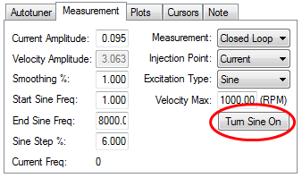
-
Turn Sine On: This button allows the user to excite the system at a single sine frequency. When this button is pressed, it grays out boxes that do not apply. You may change the sine frequency and amplitude. To stop the sine excitation, click Turn Sine Off. Turn Sine On is only visible and applicable in Sine measurements.
-
-
When the sine excitation is used on low resolution encoders, high frequency excitation may cause less than 1 count of encoder movement. If this occurs, no movement is detected on the motor for that excitation frequency. If this occurs, a data point for that frequency will not be plotted, as this results in a calculation of 0dB for gain and -infinity for phase.
Plot Options
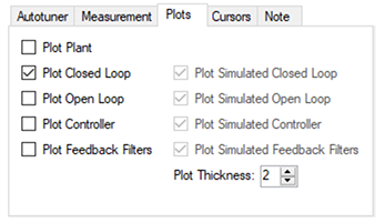
By default, only the measured closed loop plot is selected. You can control which of these responses are displayed on the Bode plot by checking or unchecking the Plot Plant, Plot ClosedLoop, Plot Open Loop, Plot Controller, and Plot Coherence check boxes shown. The options Plot Simulated Closed Loop, Plot Simulated Open Loop, Plot Simulated Controller, and Plot Simulated Feedback Filters are only available in Bode plot mode, not PST mode. The Plot Thickness setting controls the thickness of the line(s) in the Bode plot.
Coherence
The coherence option is only available for noise and PRB measurements; it is not available for Sine excitation measurements.
Coherence is an indicator of how accurate your data is. For example, 0 dB (1 in linear numbers) means you have perfect coherence. Another way to think of this concept is that for one unit of input, you get one unit of output. Coherence is calculated as follows:
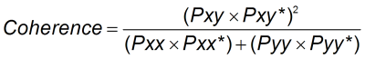
where:
Pxx = Power Spectral Density of Input signal
Pyy = Power Spectral Density of Output signal
Pxy = Cross Spectral Density of Input and Output
* designates complex conjugate
Cursors
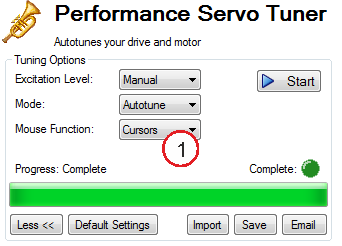
Enabling cursors allows you to note specific points of interest on the Bode plot and create a table of reference points in the summary table. To enable cursors, choose Cursors from the Mouse Function drop-down(1).
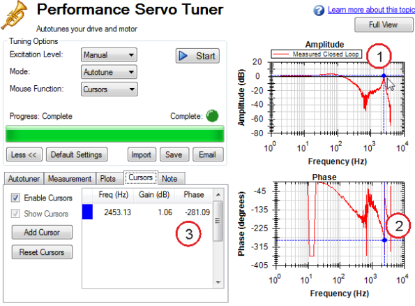
To move the cursor, move your mouse over the cursor in either the Amplitude (1), or Phase (2) plots, click and hold the left mouse button, and drag the cursor to a new location. Notice as you drag the mouse, the Frequency, Gain and Phase change in the summary window (3).
To add more cursors, click Add Cursor; you can add 10 cursors to the Bode Plot. When selecting a cursor, the cursor closest to the mouse will be selected. While dragging the cursor, the cursor will snap to the closest trace on the plot.
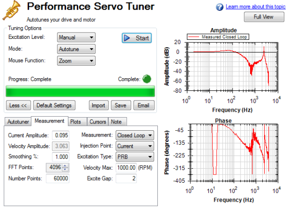
When cursors are enabled, zoom functions on the graph are disabled. To re-enable zooming, switch the Mouse Function to Zoom.
The dotted crosshair lines are only drawn for the active cursor selected; to remove all cursors from the screen, but retain their position, uncheck Show Cursors . To reset all cursors, click Reset Cursors.
To restore the scale of the graph to the default setting after zooming in, right-click on the graph and select Set Scale to Default.
Note: If a .CSV file is saved or emailed after placing a cursor on the Bode plot, a cursor summary is included in the .CSV raw data.
Resizing Bode Plots
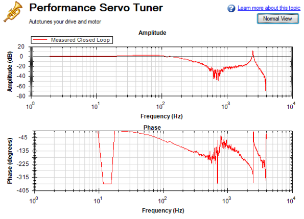
In the PST view, the Full View and Normal View button (1) in the upper right of the window allows you to see the Bode Plot in greater or less detail. When viewing the Bode Plot in full view, the PST settings are hidden behind the Bode Plot. To access the PST settings, click the Normal View button in the upper right of the window.
Simple measurement normal view
Simple measurement full view
Reading and Understanding the Bode Plot
You can operate the PST without understanding how to read a Bode plot; however, understanding Bode plots will help you to use more advanced tuning techniques, which are covered more in depth in the Tuning Guide documentation.
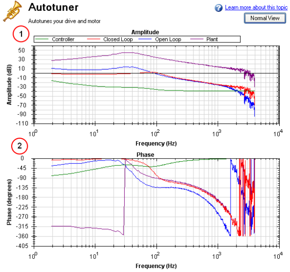
Four Bode plot traces are displayed by default:
- Controller (green): This trace represents the frequency response of the tuning in the velocity loop and position Loop, this trace also includes anti-resonance filter 1 and 2 (also referred to as [C]).
- Closed loop (red): This trace shows the frequency response of G/(1 + G * H) where G = C * P, and H is the frequency response of anti-resonance filters 3 and 4.
- Open loop (purple): This trace shows the frequency response of G * H, where G = C * P, and H is the frequency response of anti-resonance filters 3 and 4.
- Plant: This trace shows the frequency response of the mechanics of the drive and motor (also referred to as [P])
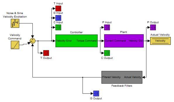
The diagram of the velocity loop on the drive below explains the frequency response that each of these traces represents:Tuning Guide
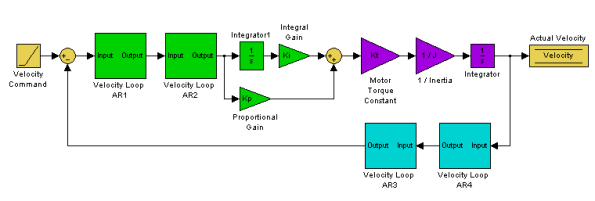
These blocks can be grouped into Controller, Plant, and Feedback sections:
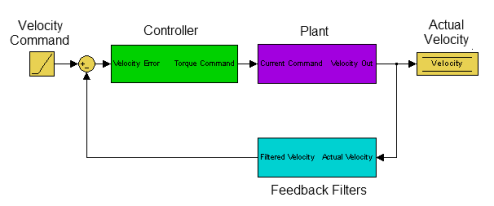
All of the green blocks have been grouped together to create the Controller [C]. The Controller is the portion of the control loop containing all velocity and position loop tuning, including the forward path filters.
All of the purple blocks have been combined to make the Plant [P]. The plant represents the mechanical and electrical properties of the motor, drive and any mechanical bodies attached to the
The two feedback filters have been combined into one block. This value is never measured directly; however it contributes to both the Open Loop [G] and Closed Loop [T] frequency responses.
The definition of the Open Loop [G] frequency response is:
Open Loop = Controller x Plant x Feedback Filters
The definition of the Closed Loop [T] frequency response is:
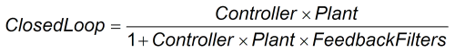
Below is a diagram of measurement points (input and output) for each of these frequency responses. The input and output markers have been color coded with the color they appear in the PST:
Current Excitation:
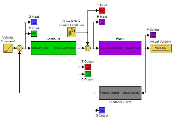
Velocity Excitation:
The resulting plots are the frequency response of output/input for each measurement.
For more information regarding these traces, please refer to the Tuning Guide documentation.
Below is a Bode plot of a motor with no
The lower plot is the phase plot (2). This plot is used in conjunction with the magnitude plot to determine stability, and helps you to understand what kind of latencies exist in the servo system, or if latencies are induced by filters in the velocity loop.
Using the Performance Servo Tuner to Manually Tune Systems
Often, you must manually adjust a control loop in order to obtain optimal machine performance. You can use the Performance Servo Tuner (PST) interface to tune your control loop for best performance. A powerful feature of the manual tuning interface is the ability to simulate the frequency response before it is measured. This feature allows the user to take a base measurement, disable the motor, adjust tuning parameters, and simulate the frequency response of the motor without taking a new measurement. This process saves time and protects equipment from dangerous oscillations.
To begin the manual tuning process, put the Performance Servo Tuner into Bode Plot mode.
Several differences exist between PST and Bode Plot Interfaces:
- When the PST is put into Bode Plot mode, the Autotuner tab is removed from the advanced features, and replaced with a Tuning tab.
- The Plots tab unlocks simulated traces for closed loop, open loop, controller, and feedback filters.
Using the Tuning Simulation
To simulate tuning, there must be a valid Plant Plot in the PST (whether measured with a Bode Plot measurement or a full Autotune).
To select simulated plot traces, click on the Plots tab and check the following boxes:
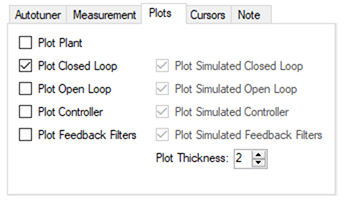
These selected boxes are the most common configuration for tuning; however, simulation will occur regardless of the check boxes selected.
The boxes on the left plot the existing frequency response of the drive based on the tuning parameters that are loaded. The boxes marked "Simulated" (on the right) use the plant data from the measurement and the tuning parameters in the PST to simulate the performance of those tuning parameters without loading them to the drive.
Using the Performance Servo Tuner Manual Tuning Interface
To use the PST manual tuning interface, click on the Tuning tab.
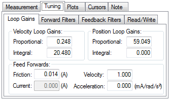
This tuning interface loads the tuning parameters on the drive each time a measurement is taken. Tuning parameters are split up into Loop Gains (Velocity Loop, Position Loop), Forward Path Biquad Filters, and Feedback Path Biquad Filters.
After modifying tuning gains, you must click on the Read/Write tab and click the Write Tuning button.
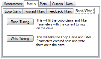
To restore the tuning on the drive to the PST interface, click the Read Tuning button.
Note: If tuning gains are modified and a Bode Measurement is made without clicking the Write Tuning button, the PST will overwrite the tuning gains in the interface with the tuning parameters on the drive.
Simulating Modified Loop Gains with the Performance Servo Tuner
Here is the frequency response of a test system after using the PST.
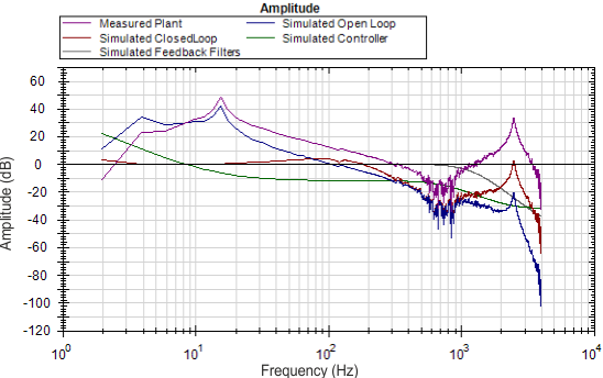
The Velocity Loop Proportional gain here is 0.248. If an application did not need to be tuned as stiff as this, then you could use the PST simulator to detune the motor to the desired bandwidth. A followup Bode Measurement can verify that the simulated response is correct.
Use the boxes in the Loop Gains tab to change tuning gains until the desired frequency response is achieved.
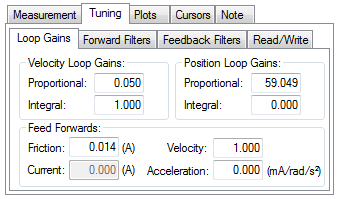
The de-tuning of velocity loop proportional and integral gains simulated that the bandwidth of the servo has been detuned from ~100 Hz to ~30 Hz.
Next, write the tuning parameters to the drive using the Write Tuning button on the Read/Write tab.
Now, complete a Bode Plot measurement to compare the simulated result with the new measured result.
The new measured Bode Plot indicates we achieved slightly lower than 30 Hz bandwidth. The servo is stable, and tuning can be refined until desired performance is reached.
Simulating Filters with the Performance Servo Tuner
Resonances add many challenges to tuning a servo. Using the correct filter in an application can greatly improve system performance when resonances are present.
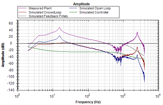
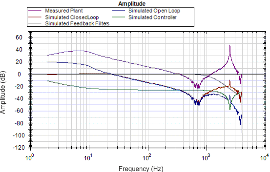
The Bode plot in this example shows a sharp, high-magnitude resonance at 2500 Hz. Because this is the only resonance, this is an indicator that a resonator (a tunable notch) filter may increase performance.
Click on the Forward Filters tab:
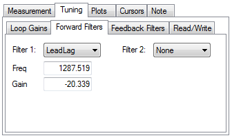
The results of the autotune are still on the drive, and provide adequate tuning. A lead lag filter is the default tuning filter, and is a good general case filter for most servo loops.
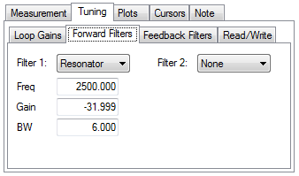
Because this test fixture has such a prominent single resonance, we can improve performance (and reduce noise) by placing a notch filter at this resonance.
By tuning a Resonator to best cancel the resonance in the plant, the resonance in the open loop, and therefore the closed loop can be minimized.
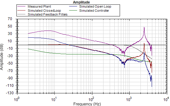
The resulting frequency response using the above resonator configuration is shown below:
Notice the attenuation of the resonance in the blue and red traces (open loop and closed loop, respectively).
Using Filters to Reduce Noise
To reduce noise, it is best to place filters in the feedback path. This placement attenuates the noise resulting from a noisy encoder being amplified by the current loop. This noise can be filtered by a forward path filter, however if a filter is placed in the forward path that introduces phase lag (like a lowpass), then your motion profile will exhibit that phase lag in the command signal. If the filter is placed in the feedback path, this lag will be avoided.