|
General Information |
|
|---|---|
|
Type |
R/W Parameter |
|
Description |
Sets the natural frequency of the pole (denominator) of anti-resonance (AR) filters 1, 2, 3, and 4; active in opmodes 1 (velocity) and 2 (position) only. |
|
Units |
Hz |
|
Range |
5 to 5,000 Hz |
|
Default Value |
500 Hz |
|
Data Type |
Float |
|
See Also |
VL.ARPQ1 TO VL.ARPQ4 on pg. 1, VL.ARZF1 TO VL.ARZF4 on pg. 1, Sets the Q of the zero (numerator) of anti-resonance filter #1; active in opmodes 1 (velocity) and 2 (position) only. on pg. 1 |
|
Start Version |
M_01-02-00-000 |
| FieldbusA Fieldbus is an industrial network system for real-time distributed control (e.g. CAN or Profibus). It is a way of connecting instruments in a plant design | Index/Subindex | Object Start Version | |
|---|---|---|---|
| M_01-02-00-000 | |||
Description
VL.ARPF1 sets the natural frequency of the pole (denominator) of AR filter 1. This value is FP in the approximate transfer function of the filter:
ARx(s) = [s²/(2πFZ)² +s/(QZ2πFZ) + 1]/ [s²/(2πFP)² +s/(QP2πFP) + 1]
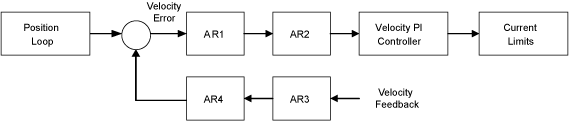
The following block diagram describes the AR filter function; note that AR1 and AR2 are in the forward path, while AR3 and AR4 are applied to feedback:
AR1, AR2, AR3, and AR4 are used in velocity and position mode, but are disabled in torqueTorque is the tendency of a force to rotate an object about an axis. Just as a force is a push or a pull, a torque can be thought of as a twist mode.
Discrete time transfer function (applies to all AR filters)
The velocity loop compensation is actually implemented as a digital discrete time system function on the DSP. The continuous time transfer function is converted to the discrete time domain by a backward Euler mapping:
s ≈ (1-z-1)/t, where t = 62.5 µs
The poles are prewarped to FP and the zeros are prewarped to FZ.
Related Topics
|
Stay Connected with Kollmorgen       
|
Copyright © 2015 Kollmorgen™ |

|