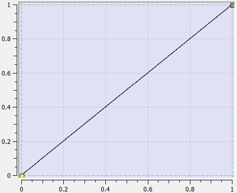
CAM Profile Segments
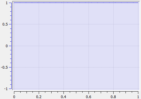
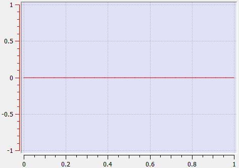
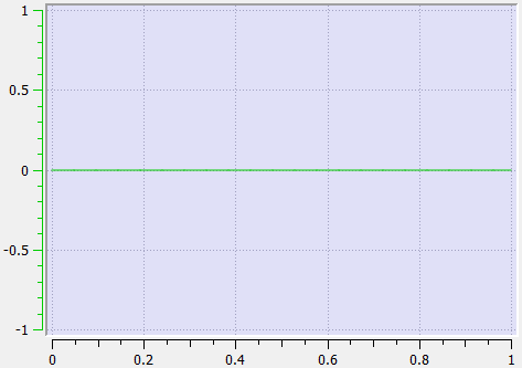
Line Segment Type
|
Segment Curve |
Velocity |
Acceleration |
Jerk |
|---|---|---|---|
|
|
|
|
|
|
Supported by |
|
|
Continuous Velocity |
|
|
Continuous Acceleration |
|
|
Interpolation Method |
Linear function: f(x) = Ax + B |
|
Advantages |
|
|
Disadvantages |
Profiles can result in discontinuous velocities. |
Parabolic Segment Type
|
Segment Curve |
Velocity |
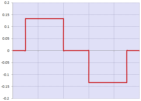
Acceleration |
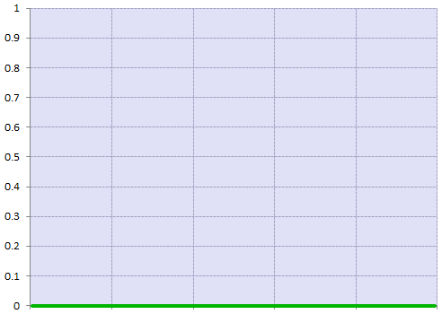
Jerk |
|---|---|---|---|
|
|
|
|
|

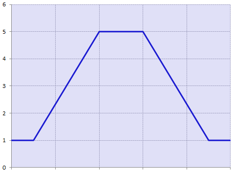
In the example:
- The blue line represents the linear (constant velocity) part of the segment.
- The black lines represent the parabolic (constant acceleration) parts of the segment.
|
Supported by |
|
|
Continuous Velocity |
|
|
Continuous Acceleration |
|
|
Interpolation Method |
Linear function: f(x) = Ax + B
|
|
Advantages |
|
|
Disadvantages |
Acceleration is discontinuous which can lead to additional electrical stress on the drives and motors. |
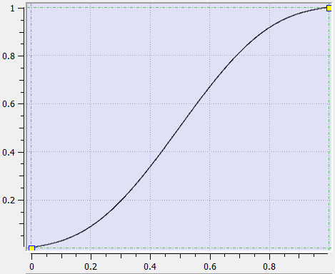
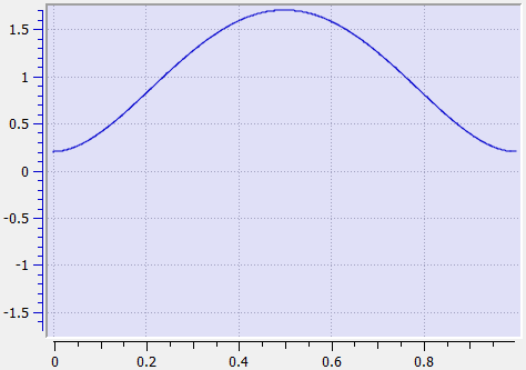
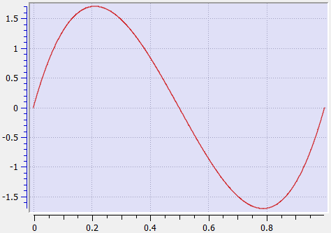
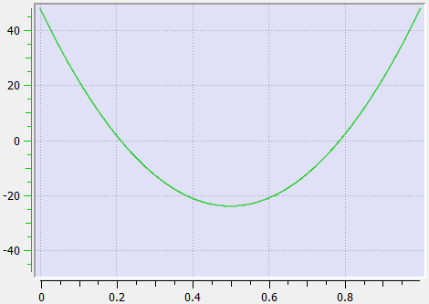
Point Segment Type
|
Segment Curve |
Velocity |
Acceleration |
Jerk |
|---|---|---|---|
|
|
|
|
|
|
Supported by |
|
|
Continuous Velocity |
|
|
Continuous Acceleration |
|
|
Interpolation Method |
5th order polynomial: f(x) = Ax5 + Bx4 + Cx3 + Dx2 + Ex + F |
|
Advantages |
With only a few segments, this type can be used to define profiles with continuously changing accelerations. Example: Sinusoidal profiles can be emulated with 6 to 12 point segments. |
|
Disadvantages |
|
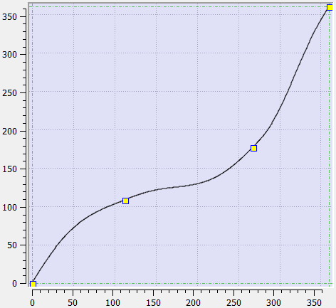
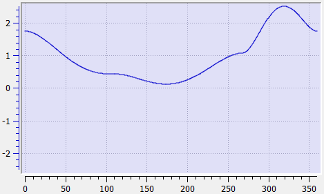
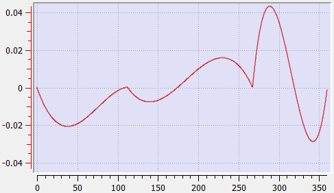
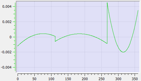
Spline Segment Type
|
Segment Curve |
Velocity |
Acceleration |
Jerk |
|---|---|---|---|
|
|
|
|
|
|
Supported by |
|
|
Continuous Velocity |
|
|
Continuous Acceleration |
|
|
Interpolation Method |
3rd order polynomial: f(x) = Ax3 + Bx2 + Cx + D |
|
Advantages |
|
|
Disadvantages |
Since only positions are specified, the user has less control over the velocities and accelerations that occur throughout the profile. |