Practical Application: Using Trace Time To Measure CPU Load
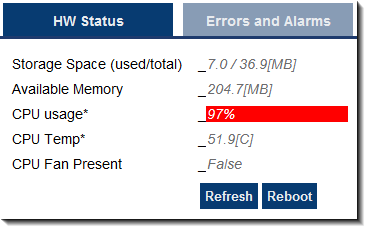
To determine the overall controller CPU usage, look at the HW Status tab on the Diagnostics page of the controller's web server.
-
- The technique to measure the CPU load is similar but the load limits change with the:
Single and dual-core AKD PDMM / PCMM.
Quad-core PCMM2G.
See Also
- Oscilloscope Control Panel about the trace times.
- Check the Peak Times
- Tasking Model / Scheduling
- CPU Load Reduction Techniques
AKD PDMM / PCMM
- If the CPU usage is:
PCMM2G
- The CPU usage alone may not provide an accurate indicator of the Motion and PLC CPU usage.
- This is because the CPU usage is the average of all the CPU cores.
Oscilloscope Trace Times
The IDE Oscilloscope trace times can be used to analyze the application performance on a controller or programmable drive.
This section describes techniques used to interpret the trace times to examine the real-time performance.
There are two major parts to consider when evaluating total performance:
- Real Time: EtherCAT + Motion Engine + PLC program.
- Non-Real Time: Everything else (the background tasks).
The Oscilloscope trace times provide a very good tool to examine the Real Time response.
- Although it doesn’t provide the complete system picture, it is a good place to start.
- It can provide some indication about the Non-Real Time load.
- However, the best indicator is the overall CPU usage and the Controller Log messages.
You need to know the Cycle Time for the system.
From the Project View, select the EtherCAT view and the EtherCAT Master Settings tab.
The update period for the system in this example is set to 250 microseconds.
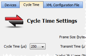
Figure 1: Cycle Time tab
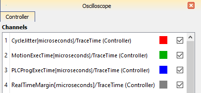
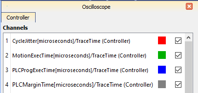
The Trace Times traces are enabled by pressing the Plug Trace Times channels button in the Oscilloscope view when your application program is running.
This button automatically configures the Channels:
|
AKD PDMM / PCMM |
PCMM2G |
|---|---|
|
Figure 2: AKD PDMM / PCMM |
Figure 3: PCMM2G |
Press the Start Button to Collect Some Data
The first thing to do is to collect data during the normal application operation, particularly once the system has reached a steady state.
Press Start and let the data collect for a few seconds and then press the Stop button.
The first traces to examine are the MotionExecTime and PLCProgExecTime.
Configure the Amplitude and Zero offset so you can see both traces easily.
This table shows some recommended values based on several Cycle Time values:
Cycle Time | Amplitude | Zero Offset |
|---|---|---|
250ms | 20 | 80 |
500ms | 40 | 160 |
1000ms | 80 | 320 |
-
-
Clearing checkboxes for the CycleJitter and RealTimeMargin or PCLMarginTime traces is useful so they don't clutter the view.
Example
This example has a Cycle Time of 250 microseconds.
- The MotionExecTime average is about 27 microseconds.
- The PLCProgExecTime average is about 68 microseconds.
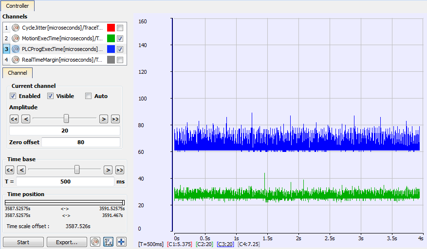
Figure 4: PLCProgExecTime and MotionExecTime
For single-core controllers, we want to investigate the combined percentage of cycle time for both the MotionExecTime and PLCProgExecTime.
- The average time for the MotionExecTime + PLCProgExecTime is 95 (27 + 68 = 95).
- This is about 38% of the cycle (95 / 250).
- This is a good value.
- This is about 38% of the cycle (95 / 250).
For multi-core controllers, we want to investigate the percentage of cycle time for each MotionExecTime and PLCProgExecTime individually.
- MotionExecTime is about 11% of the cycle.
- PLCProgExecTime is about 27% of the cycle.
- These are both good values
Check the Peak Times
The next step is to examine the spikes.
We will examine the MotionExecTim, PLCProgExecTime, RealTimeMargin or PLCMarginTime and CycleJitter traces.
- Reduce the Time base and move the traces left or right with the mouse while holding the left mouse button.
- Position the cursor to measure the peak.
In this example:
- The MotionExecTime peak is 44.
- The PLCProgExecTime peak is 89.
- This is reasonable.
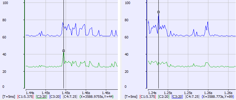
Figure 5: Peak Times
RealTimeMargin or PLCMargin Time
AKD PDMM / PDMM
To view the RealTimeMargin, configure the Amplitude and Zero offset so you can see the trace near zero.
In this example:
- The minimum (closest to zero) is 69 microseconds.
- This provides a 28% (69 / 250) RealTimeMargin (which is good).
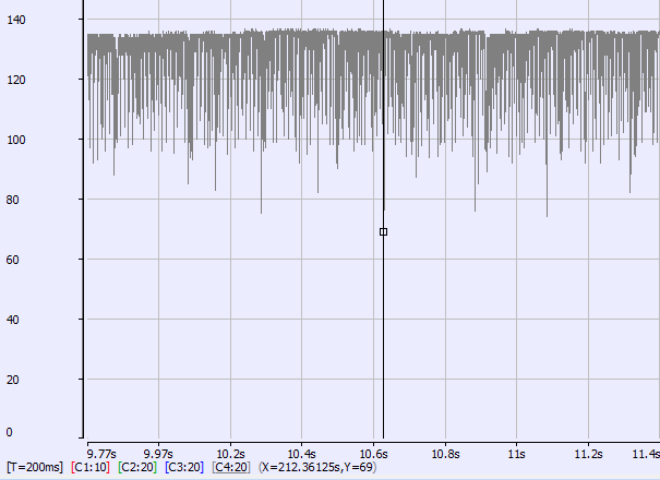
Figure 6: AKD PDMM / PDMM RealTimeMargin
PCMM2G
To view the minimum PLCMarginTime, configure the Amplitude and Zero offset so you can see the trace near zero.
In this example:
- The minimum (closest to zero) is 52 microseconds.
- This provides a 21% (52 / 250) PLCMarginTime (which is good).
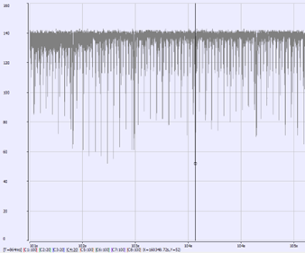
Figure 7: PCMM2G PLCMarginTime
CycleJitter Trace
For the CycleJitter trace configure the Amplitude and Zero offset so you can see the trace centered at zero.
- This trace is not too interesting unless a system is misbehaving.
- A jitter of +/-15 microseconds is acceptable.
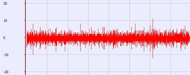
Figure 8: Cycle Jitter Trace
See Also


